Indulge me here as we veer into some summer landscaping updates! My neighbor gave me some overflow from his yard, including mint that has started to take hold. Then, thanks to some help from my parents, I was finally able to accomplish a few things in the yard that have helped me be able to start the native conversion step-by-step. First, though, I continue with some pretty ornamental annuals. We planted a Chinese hibiscus to add some curb appeal (looks like the orange? double-flowered kind) which will die back with the frost, but it is a stunner for now!
I also started a railing box with an assortment of “Superbena” colors and Salvia. They will probably all die back in the winter, but as you can see I had some fun with my first trip to a garden center; my thought was to have a red railing box to bring in the hummingbirds.
Clockwise from the top left: whiteout Superbena, “Rockin’ fuschia” Salvia, sparkling amethyst Superbena, red Superbena, Superbena royale “Romance,” and scarlet sage
Then, my bosses gave me some of their backyard overflow! I put a deck planter down to hold black-and-blue and tropical Salvia (more hummingbird magnets, hopefully). They can be prolific perennials, so I’m hoping they’ll continue to flesh out the box. I have temporarily moved the anise hyssop into the swan planter you can see below!
They also gave me mountain mint and Spigelia marilandica (which I’m actually hoping to take home to plant along my parents’ stream bed). On the porch planter side of things, though, I found a handy tip and some perfect fit rods and wood pieces to shore up the railing planters.
word of the day: shim!
My first real natives that were planted in ground went where the elephant grass was torn out. I now have a pair of summer sweet bushes in their place.
“Vanilla spice” varietal
I also got a showy varietal of black-eyed Susan, both a native and a nod to my MD roots, for the porch.
“Sunbeckia Lucia” varietal that grows happily in a porch planter. Nice because I can see the butterflies there on the porch from my home office window! Here’s a broad-winged skipper enjoying a nectar meal.
Between all of these, I have been thrilled to watch the skippers (and other pollinators) parade in. It is pretty rewarding to watch them find the native flowers, and there will be much more to come…likely shovel by shovel!
Many thanks to Jonathan Chang for getting me most of the way to this goal! I am sharing some details of the process of identifying the URL here. Check out the linked tutorial; I am illustrating some of the steps to get to where you can find the API.
Right-click on the Story Map web page and select “Inspect”
Select the “Network” tab in the console
Filter by “Fetch/XHR”
Refresh the page
Scroll down to the layer you want, and watch for “FeatureServer” in the “Name” field
Right click this entry, “copy URL” and paste into the browser, and delete the string including and after the ?
This should get you to the API where you can see the layer list; is your layer of interest there? If so, it is followed by a number in parentheses. Click on it, and this is the URL you can use with the esridump tool
Well, good thing I went out to take pics of the grass panicles in my yard because the guy came to cut it today. Ultimately want to be lawn free, and the good news is, I didn’t find any Bermuda grass! I used iNaturalist and some lawn grass ID web pages to zero in on that it appears I have Kentucky bluegrass, tall fescue and sweet vernal grass (broadly considered cool weather lawn grasses). However and unfortunately, the only place I’ve found Bermuda grass is in my potted plants. This is likely due to that I supplemented my potting mix with the fill dirt that contractors brought in after my water line installation. Still positive news is that it is very clay-heavy and outside, not much is growing in that stretch (including Bermuda grass). I bet there’s a seed bank in there sadly. Yet, it hasn’t made much of a move this year, and let’s hope it stays that way.
Create a Google Earth Engine account: get to the place of where you can login to the coding console. If you use the package to help you get setup with an account, it will not take you through the final step(s). I went through this process while creating a new account, and though there is currently a bug with authentication, this was causing me more headaches than I was realizing.
Setup a conda environment (I used miniconda):
create and activate your environment
install python
conda install numpy
conda install earthengine-api==0.1.370
Install the following dependencies if you don’t already have them. You also might run into a bear of a problem with protobuf, protoc, libprotoc etc. If so, activate your conda environment and roll back protobuf to pip install protobuf==3.20.3
gdal-bin
libgdal-dev
libudunits2-dev
Edit your ~/.Renviron file to include the following (or create it if it doesn’t exist): RETICULATE_PYTHON="path to your conda env python install" RETICULATE_PYTHON_ENV="path to your conda env"
Install reticulate R package
Install rgee R package
use install_ee_set_pyenv() with your environment settings as above
ee_Authenticate()
This should get you to the point of having rgee run off your own custom Python environment, with the downgraded version of the Earth Engine API required to authenticate at the time of this writing. A workaround for the bug in initializing GEE is starting your script as follows (bypassing ee_Initialize()): library(rgee) ee$Initialize(project='your project name')
You will also have .Renviron entries for Earth Engine now. This final step is one I’m unsure of: if you haven’t manually created a legacy asset folder, you may from here be able to run ee_Initialize() and create one. I had created one, and so I got caught in a loop of it saying it already existed while wanting me to create one. So, in short, I’ve never really been able to successfully run ee_Initialize() and the package author is at a point of not even wanting to maintain it anymore. The problem here is that you don’t get this file generated: .config/earthengine/rgee_sessioninfo.txt
So, you can make your own structured as so:
“user” “drive_cre” “gcs_cre” “YOUR GOOGLE USERNAME” “PATH TO GOOGLE CREDENTIAL FILE” NA
The path to your credential file is the one you created to authenticate earth engine, somewhere in that folder. (Save a copy elsewhere to to move back into that path, because I’m not sure the file persists between sessions.)
I start this as a placeholder blog annually to keep track of bird sightings and dates, to summarize at the end of year! Today it truly begins…
4/6 – I dragged my non-birder beau up the Hillview Natural Trail (and through the paved trail) at Eisenhower Park (San Antonio, TX) to get a glimpse of my lifer golden-cheeked warbler!
5/17- Josh Gant found an incredible record of common swift at the Meadows, during the spring festival! What a crowd-pleaser, to say the least!
…more to come…and to be fully fleshed out in a NYE post!
It appears that the last MD pelagic to have a great skua this month was Mar 1 1992 and there were 2 birds seen then! Notes variably place the records at Elephant’s Trunk and near Baltimore canyon, but all records appear to be during a 12 hr trip. Similarly, there were several birds per trip in the 70s. On Mar 15 1996, there’s a record from a Montauk pelagic, and the Mar 4 1995 notes are one of my favorites:
Life bird. Adult; 63 miles out, at north end of Block Canyon. Most-wanted species by most on this trip. We approached a trawler and started chumming. The bird appeared out of nowhere, circled the chum slick, dove on a few gulls, then began picking up its own fish in the slick. From JA’s notes: The Great Skua was found amongst hundreds of GBBGs, lesser numbers of HERGs, and about 15 NOFUs that were loitering around a commercial trawler. After “stealing” the birds from the trawler, we watched the beast for about one half hour and then finally left it.” Much jubilation ensued.
I thought it was only fitting to adorn the title of today’s post with the icon of the month! My heart was warmed by scores of alcids today! I stuck with pretty much the layer formula that works for me:
Eddie Bauer duffel coat (below the knee 650 down parka)
Faux fur hat with ear flaps and chin strap
Cape May whale watch & research center buff (represent!)
Down knee-length vest
Heaviest smart wool base layer
Outdoor fleece-lined leggings (Avalanche)
Arctic muck boots
Weather-proof gloves
Hand warmers
Costa sunglasses
This time I tried my heated socks, but the battery on one of them is faulty, and the other didn’t last the whole day. So, I’m going back to my Comrad wool compression socks; they did the job last time so I shouldn’t have veered. Also, I’m going to look for cold weather convertible mitten gloves next time.
As I psych myself up for yet another pelagic season in the north Atlantic, I review this month’s “nearby” skua sightings. On Valentine’s Day 1991, be still my heart: it appears a record from shore at Manasquan inlet NJ (among others that year) was accepted to genus level. Other encouraging records:
Feb 19 1995: This was a day trip that left from Cape May and encountered a great skua at 19 fathom seamount off DE I’m curious about what appears to be a very early departure time. I wonder if we could swing or would consider that for our current trips, and of course what difference it makes?
Feb 26 1995: This was another day trip that appears to have gone out of MD, but for what it’s worth (if anything) we sometimes eek into MD waters
various records before my time at the MD pelagic general hot spot: the most enticing details here are the number of birds recorded on trips in the 70’s!
Valentine’s Day 1982
Feb 1 1976
Feb 9 1975
Feb 7 1975
Feb 2 1975
Feb 1 1975: a total of *9* birds are reported 67-111 km E of Ocean City
Feb 3 1974
So yet again, I budget for a ticket and get my seasickness medication in order to plan for more days at sea…
This year, my “big birding vacation” was that I signed up for a dream trip in the form of Kansas lek treks! On 4/14 I visited a lesser prairie-chicken lek and got to start the morning with some dancing chickens. The afternoon would see a possible tough miss of unpreparedness, where flying by the seat of my pants, I didn’t learn the thick-billed longspur song. I may have heard one birding my way to Garden City, but I console myself with that it stopped singing and I was never able to find the unknown bird. The next day was pretty magical though: I made it into mountain time to see a scaled quail perched up on a fence post in the early light. It was truly lucky because perhaps in part due to the awful weather, it was the only one I saw, and never reappeared once it flushed. I also am pretty sure I heard a Cassin’s sparrow, but it never sang again, and everything was hunkered down as the windy cold rain set in.
Migration would kick off with me getting to hear a Cerulean warbler for the first time in years! We’d also get some “backyard” excitement with a very red curlew sandpiper right at the meadows mid-May! The most fun part of this bird was doing a true from work chase, where a coworker got it as a lifer and we all got to bond over a rarity convergence.
I then would get to see a great birder friend that now lives a country away twice this year in NJ! She would have to put up with me being sick the first visit, and the 2nd came at a very busy time…but, we carved out some quality time to hang and look at birds nonetheless!
My next lucky 24 hours would come on an incredible pelagic weekend! I was able to race up to Brig to see a bar-tailed godwit on 6/18 before turning right around to finish packing ahead of boarding the boat that night. The next day, on our way back near Elephant’s Trunk(!) an obliging South Polar skua made a slow pass right in front of the boat. My lifer was once again celebrated with the friends I’ve made over these many boat trips, including the crew of the Cape May Whale Watch & Research Center (can’t say enough good about these trips, and excited to take my next venture early in the new year…get signed up!).
On 7/2 the recurrence of a little egret at Bombay Hook would bring some excitement to the summer doldrums. I made a round trip go of it, driving around to get there early and then taking the ferry back. The latter half of the year, I was thankful to be asked to guide for the Cape May fall festival! I got to guide and bird with old friends, and meet some new ones! As always, a chaotic and wonderful weekend greeted us with the unexpected and plenty of enthusiasm from all involved.
The onset of winter birding would be heralded by a black guillemot irruption, and on 11/5 I got to see this much-wanted lifer. It left me with the mark of the beast on my eBird lifer tally (ha! …an incomplete life list though, as there are many Costa Rican birds from my 1st trip that aren’t recorded there). So, I was itching to put an new bird in the books…and what a bird that would be! The really wacky lifer of the year for many of us would be the red-flanked bluetail that I finally got to see on 12/22.
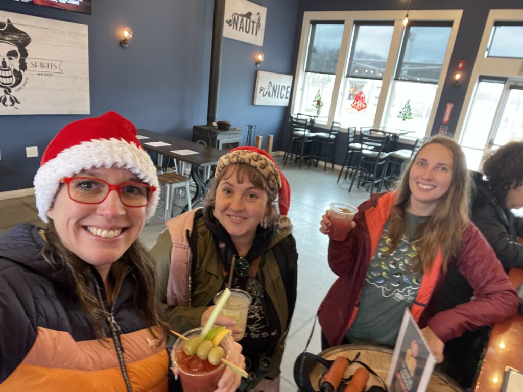
On 12/17 I was honored to take on section 3SE of the Cape May CBC, and got to spend the day birding with and among some of my best friends of south Jersey!
Yes, Nauti spirits was in our section, and this was completely necessary for access to their grounds…photo credit: Kelly Ball
Incredibly 2023 still had some bang left in it as I closed out the year in FL. I waded through the inaccurately named “dry bones trail” of the Cape Coral rotary park to hear my nemesis mangrove cuckoo on 12/29! The water was too deep for me to get through the connector with the boots I had (knee-high wellies would have done the trick). But, just on the other side on the mangrove alcove trail, some lucky birders got great looks the following day! (I never would catch a glimpse, but, next year goals…) I also always enjoy getting to see the Florida subspecies of red-shouldered hawk. Also in the realm of neat color morphs that show up in FL, I got to see the “great white heron!” My final lifer of year was a true New Year’s Eve last min bird: American flamingos still hanging out, presumably, from the hurricane displacement on a sand bar. My mom, a family friend and I went on a the afternoon dolphin & wildlife cruise which left at 1:30 PM to see them, which overall was just a great way to spend the last day of 2023.
Happy new years…and as usual…what will 2024 bring us?!
We are just getting back from an incredible night and day at sea! From land, temps bottomed out at 57F and got up to a high of 79F. We started the morning at ~90 mi offshore off Wilmington canyon and worked our way back in from there. Here’s what I wore to stay comfortable…
parka (yes really! made for a great blanket early in the day)
UPF pullover hoodie
visor
Costa del Mar sunglasses
tee shirt
cotton leggings
flipflops
I wish I would have brought my hooded puff layer. I didn’t use my trucker hat, bucket hat or buff, but always good to have them on board, in addition to wind stopper gloves.