Here’s a script that loops over climate NetCDF bricks in a folder and extracts the values for each layer in the brick of each file, in this case averaged over polygons in a shape file.

rm(list = ls())
library(raster)
library(rgdal)
library(ncdf4)
library(reshape2)
library(stringr)
library(data.table)
setwd("where your climate files are")
your_shapefile <- readOGR("path to your shapefile","the layer name for your shapefile")

climate <- rbindlist(lapply(list.files(pattern="nc"), function(climate_file)
{
#in my case, the weather variable is in the filename
climate_var = ifelse(grepl("pr",climate_file),"pr",ifelse(grepl("tmax",climate_file),"tmax","tmin"))
print(climate_var)
climate_variable <- brick(climate_file,varname=climate_var,stopIfNotEqualSpaced=FALSE)
#I needed to shift the x-axis to be on a -180 to 180 scale
extent(climate_variable)=c(xmin(climate_variable)-360, xmax(climate_variable)-360, ymin(climate_variable), ymax(climate_variable))
blocks <- spTransform(blocks,projection(climate_variable))
r.vals <- extract(climate_variable, blocks, fun=mean,na.rm=TRUE,df=TRUE,layer=1,nl=1680)
r.vals <- melt(r.vals, id.vars = c("ID"),variable.name = "date")
r.vals$climate <- climate_var
#depending on the filename convention of your files, get a variable for your climate model and name it "modelname"
r.vals$model <- modelname
climate_variables[[length(climate_variables)+1]] <- r.vals
}))

climate <- rbindlist(climate_variables)

At this point, you have a data frame called “climate” that has all your data long-form. You can cast this as you see appropriate depending on your needs!

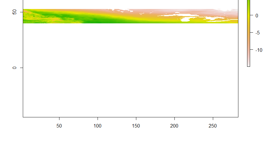
I can’t be thankful enough for my godsend Twitter friend/NetCDF guru Michael Sumner for coming in clutch to rectify this problematic file! As I take my baby steps in learning how to deal with NetCDF files (~3 weeks after being thrown into the “deep end” and trying to tread water), I realized that one of our files had some sort of problem. Relevant to this issue, NetCDF files are often (not always) multidimensional arrays, where 2 of the dimensions are coordinates. The variables can be defined in relation to the dimensions of the file. So for instance, in my case, temperature is described over space and time (4-dimensional array), and each temperature value corresponds to a location and time. So, each temperature value “goes along with” a set of coordinates and a time. When I imported the NetCDF file as a raster brick (which means I put the array data into a stack of grids), the metadata seemed to show a larger longitudinal “step” than latitudinal, the latter of which was at the correct resolution. Note that this means, as is common, I took what is really a point (a temperature value corresponding to a latitude, longitude and time) and turned it into a grid, where the original point is the center of the resulting cell that gets the value. I tried  plotting it to see what it looked like.

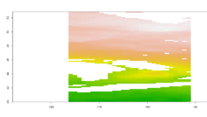
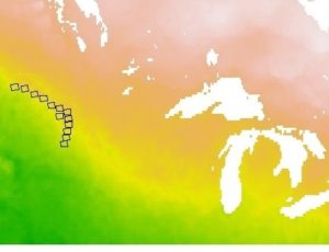
I tried to crop the image to only the extent I needed but it still was messed up.

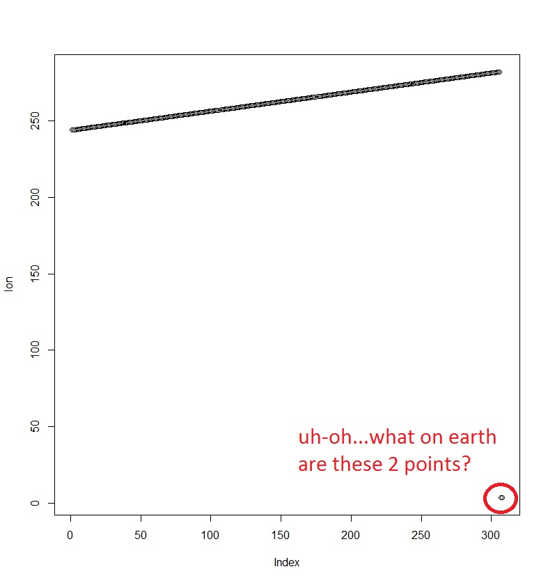
I took this at face value, that perhaps the grid was somehow “wrong,” but my new friend showed me how to look more deeply into the problem! He opened the file in R and extracted the coordinate values, plotting for a visual diagnosis of the problem.

library(ncdf4) con <- ncdf4::nc_open("file.nc")
lon <- ncdf4::ncvar_get(con, "lon")
lat <- ncdf4::ncvar_get(con, "lat")
ncdf4::nc_close(con)

So, my friend suggested plotting the longitude values stored in this dimension of the array.

Herein we start to see a problem! Something is off about the longitudes stored in the array.

head(lon)
# [1] 244.0625 244.1875 244.3125 244.4375 244.5625 244.6875
tail(lon)
# [1] 281.8125 281.9375 282.0625 282.1875 3.5200 3.5100
r <- raster::brick(f, stopIfNotEqualSpaced = FALSE)
extent(r)
# class : Extent
# xmin : 3.056128
# xmax : 282.6414
# ymin : 40
# ymax : 52.875

## let's treat it as if the start is correct,
## the final two columns are incorrect
## we hard-code the half-cell left and right cell edge
## (but note the "centre" might not
## be the right interpretation from this model, if we're being exacting)
valid_lon2 <- c(lon[1] - 0.125/2) + c(0, length(lon)) * 0.125
valid_lat <- range(lat) + c(-1, 1) * 0.125/2
r2 <- setExtent(r, extent(valid_lon2, valid_lat))
r_final <- raster::shift(r2, x = -360)

Another problem I ran into: apparently Nov-Dec. 1999 monthly averages for HADCM3 B1 precipitation, where I flipped the axes in NCO, are blank.

problem <- brick("hadcm3.b1.pr.NAm.grid_monthly.nc_out.nc")
plot(problem$X1999.11.15)
plot(problem$X1999.12.16)

The above returns the correct axes, but blank plots. The problem is present before I flipped the axes, so I have to go back to the original files before I did the averaging to find out what’s wrong. I wonder if there were blank layers anywhere in the Nov-Dec daily data?

From a THREDDS server, I’m using the NetcdfSubset portal to obtain a spatial subset of my climate data set of interest. Since the files I need are too big to download from their HTTP server, they instead give me an OPeNDAP URI with the spatial subset info. I then pass that to nccopy from the NetCDF library.

Then, I installed CDO and wrote a script to do the monthly means for all the files: it averages a daily time step file into a monthly averaged (or whatever metric you choose) file.

cdo monmean foo_hourly_or_daily.nc  foo_monthly_mean.nc

Then, I installed nco to flip the axes.

ncpdq -a lat,lon in.nc out.nc

Then, I imported the correctly-oriented files into R.

rm(list = ls())
library(raster)
library(rgdal)
library(ncdf4)
setwd("wherever your files are")
climate <- brick("filename.nc",varname="whatever your climate variable is")

In my case, as I think is common for climate files, longitude was on a 0-360 scale, instead of -180/180.

I ended up getting a bunch of climate NetCDF files from a colleague for each combination of climate model, climate change scenario and variable. So, what I have is a list of 3-D files consisting of observations/predictions of a given weather variable over latitude, longitude and time (you can picture them as cubes, if you like). I will need to spatially adjust the files, and then subset the data.

ncpdq -a lat,lon in.nc out.nc

I need to…

• keep only the extent within a shape file we’re using
• figure out how to summarize it by the polygons in the shape file
  • average?
  • keep only the center point?

Some of my closest colleagues, Brooke Bateman and Andy Allstadt, had some good advice for how to work with the netCDF files in R once I get them:

• ncdf4 package
• raster package: can open netCDF either as…
  • single layer (with the raster function)
  • the entire thing (brick function)
• SDMTools
  • sample x,y points from raster using extract data function
  • convert the raster to ASCII

You can load those libraries, and then do a few things to take a look.

library(<span class="pl-smi">raster</span>)
print(raster(<span class="pl-s"><span class="pl-pds">"</span>afile.nc<span class="pl-pds">"</span></span>))  <span class="pl-c">## same as 'ncdump -h afile.nc</span>
b <- brick(<span class="pl-s"><span class="pl-pds">"</span>afile.nc<span class="pl-pds">"</span></span>, <span class="pl-v">varname</span> <span class="pl-k">=</span> <span class="pl-s"><span class="pl-pds">"</span>pr<span class="pl-pds">"</span></span>) #this is the variable name internal to the file