Best Birds of 2023

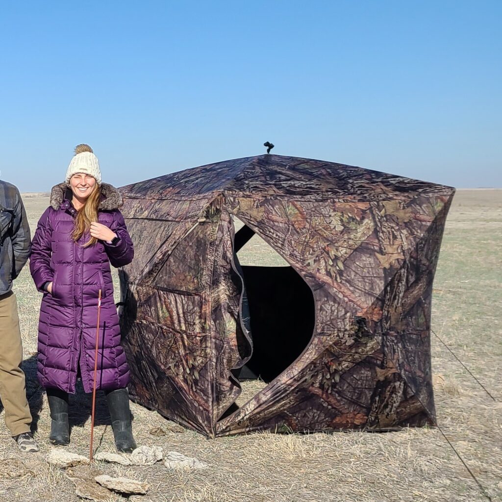
This year, my “big birding vacation” was that I signed up for a dream trip in the form of Kansas lek treks! On 4/14 I visited a lesser prairie-chicken lek and got to start the morning with some dancing chickens. The afternoon would see a possible tough miss of unpreparedness, where flying by the seat of my pants, I didn’t learn the thick-billed longspur song. I may have heard one birding my way to Garden City, but I console myself with that it stopped singing and I was never able to find the unknown bird. The next day was pretty magical though: I made it into mountain time to see a scaled quail perched up on a fence post in the early light. It was truly lucky because perhaps in part due to the awful weather, it was the only one I saw, and never reappeared once it flushed. I also am pretty sure I heard a Cassin’s sparrow, but it never sang again, and everything was hunkered down as the windy cold rain set in.

Migration would kick off with me getting to hear a Cerulean warbler for the first time in years! We’d also get some “backyard” excitement with a very red curlew sandpiper right at the meadows mid-May! The most fun part of this bird was doing a true from work chase, where a coworker got it as a lifer and we all got to bond over a rarity convergence.

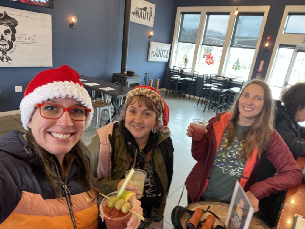
I then would get to see a great birder friend that now lives a country away twice this year in NJ! She would have to put up with me being sick the first visit, and the 2nd came at a very busy time…but, we carved out some quality time to hang and look at birds nonetheless!

My next lucky 24 hours would come on an incredible pelagic weekend! I was able to race up to Brig to see a bar-tailed godwit on 6/18 before turning right around to finish packing ahead of boarding the boat that night. The next day, on our way back near Elephant’s Trunk(!) an obliging South Polar skua made a slow pass right in front of the boat. My lifer was once again celebrated with the friends I’ve made over these many boat trips, including the crew of the Cape May Whale Watch & Research Center (can’t say enough good about these trips, and excited to take my next venture early in the new year…get signed up!).

On 7/2 the recurrence of a little egret at Bombay Hook would bring some excitement to the summer doldrums. I made a round trip go of it, driving around to get there early and then taking the ferry back. The latter half of the year, I was thankful to be asked to guide for the Cape May fall festival! I got to guide and bird with old friends, and meet some new ones! As always, a chaotic and wonderful weekend greeted us with the unexpected and plenty of enthusiasm from all involved.

The onset of winter birding would be heralded by a black guillemot irruption, and on 11/5 I got to see this much-wanted lifer. It left me with the mark of the beast on my eBird lifer tally (ha! …an incomplete life list though, as there are many Costa Rican birds from my 1st trip that aren’t recorded there). So, I was itching to put an new bird in the books…and what a bird that would be! The really wacky lifer of the year for many of us would be the red-flanked bluetail that I finally got to see on 12/22.

On 12/17 I was honored to take on section 3SE of the Cape May CBC, and got to spend the day birding with and among some of my best friends of south Jersey!

Yes, Nauti spirits was in our section, and this was completely necessary for access to their grounds…photo credit: Kelly Ball

Incredibly 2023 still had some bang left in it as I closed out the year in FL. I waded through the inaccurately named “dry bones trail” of the Cape Coral rotary park to hear my nemesis mangrove cuckoo on 12/29! The water was too deep for me to get through the connector with the boots I had (knee-high wellies would have done the trick). But, just on the other side on the mangrove alcove trail, some lucky birders got great looks the following day! (I never would catch a glimpse, but, next year goals…) I also always enjoy getting to see the Florida subspecies of red-shouldered hawk. Also in the realm of neat color morphs that show up in FL, I got to see the “great white heron!” My final lifer of year was a true New Year’s Eve last min bird: American flamingos still hanging out, presumably, from the hurricane displacement on a sand bar. My mom, a family friend and I went on a the afternoon dolphin & wildlife cruise which left at 1:30 PM to see them, which overall was just a great way to spend the last day of 2023.

Happy new years…and as usual…what will 2024 bring us?!

Pelagic Overnight

We are just getting back from an incredible night and day at sea! From land, temps bottomed out at 57F and got up to a high of 79F. We started the morning at ~90 mi offshore off Wilmington canyon and worked our way back in from there. Here’s what I wore to stay comfortable…

  • parka (yes really! made for a great blanket early in the day)
  • UPF pullover hoodie
  • visor
  • Costa del Mar sunglasses
  • tee shirt
  • cotton leggings
  • flipflops

I wish I would have brought my hooded puff layer. I didn’t use my trucker hat, bucket hat or buff, but always good to have them on board, in addition to wind stopper gloves.

Yard Tree Candidates

From the list native to the county that would also produce some yummy fruits (for me and the birds) or add conservation value…

  • green ash – can tolerate poorly-drained (back yard)
    • https://entomologytoday.org/2016/03/07/heres-how-to-inspect-your-trees-for-emerald-ash-borer/
    • https://eab.russell.wisc.edu/signs-and-symptoms/
    • questionable native status in the county though: http://capemaywildlife.com/_templates/group_oleaceae.html
  • common serviceberry – well drained (front yard)
  • Canadian serviceberry – ditto
  • sand hickory – front yard
  • common hackberry – not picky (back yard?)
    • native status in the county disputed: http://capemaywildlife.com/_templates/group_elms.html
  • common persimmon – loamy (front yard)
  • American hollyBerryland (backyard)
  • black walnut – sandy loam (front yard)
  • eastern redcedar – well-drained but also wet (either?)
  • mountain laurel – well-drained (front yard)
  • northern spicebush – not picky, average/moist (back yard?)
  • sweetgum – logs for mushrooms if you take yours down?
  • tulip tree – well-drained (front yard)
  • southern crab apple – not picky? well-drained (front yard?)
  • red mulberrywell-drained but moist (either?)
  • American plum – not picky (back yard?)
  • black cherry – well-drained (front yard)

Compassion Fatigue

Yes, I’m writing this the day after Earth Day for a reason. I love that beautiful day we take to soak in nature in my favorite season of rebirth and new growth. However, the flip side of the appreciation that comes with being an ecologist these days seems to come with an inevitable degree of compassion fatigue. I didn’t think I’d get here, but I feel like burying my head in the sand. The bad news is overwhelming, and I can’t stomach it anymore. Maybe though, there’s a positive to this: I can’t take hearing about the things I cannot do anything about (or seemingly at least). I immediately click away from the negative environmental stories that once drew me in like clickbait; it all just brings on a feeling of hopelessness, and furthers a feeling of not being able to act meaningfully on it. I feel like I’m protecting my head, and maybe there’s a good side to focusing on the actionable, which has been an overall priority lately in my life.

Remote Sensing for Birders

Or: Birding in the era of climate change

In my previous job as a researcher, I modeled hydrology of wetlands, including the playa lakes region. Visiting Kansas this weekend was my first time getting to spend time in that region since that project concluded, but sadly, I got to see the phenomenon we were testing: what drought on the landscape looks like. So, I embarked on a quest to find water with tools that are by and large accessible to birders.

I continue my evangelism of Google Earth Engine, which has somewhat quietly changed the game of remote sensing, though maybe more loudly in today’s research landscape: I was an early adopter when it first came out and swooned over the potential. Now, I imagine it has become a much more popular research tool, but I want the floodgates to open for hobbyists too. It is a truly remarkable game changer and uprooted how we always did things (e.g. during my PhD) to process and analyze remote sensing (e.g. satellite imagery) data. These days, you can pull from a library of images straight into your coding environment and mapping output (I still get goosebumps typing that). You can query a compendium of publicly available satellite images, write your code to analyze it, and display the output in one browser tab…oh, and did I mention the excellent documentation and gobs of available coding examples?

The Quarry

On this mission, I was specifically looking for Clark’s grebe (Aechmophorus clarkii): though their habitat requirements are flexible in migration, they tend to like big wetlands or lakes with deep, persistent water. These proclivities governed what I was able to do to identify suitable water bodies.

The Solution

I devised a script (below) to leverage Sentinel imagery to calculate normalized difference water index (NDWI) which is a well-known indicator of water on the landscape. You can copy the whole script right into your code editor and run it as-is, but I’ll walk through in general what it does in the remainder of the post. I also co-opted a fair number of code chunks from the Google Earth Engine examples, so you’ll find some of these functions (e.g. the cloud mask function) elsewhere in their documentation. I commented out some map layers as well, but you can play with adding them back in.

Methodology

First, I filtered the imagery down to the state of Kansas to make the analysis relevant and manageable. Given that playas are filled by rainwater and the problem was drought, I could be a little more focused in my image gathering: I looked at the 2 weeks prior to my arrival and kept images with < 30% cloud cover. (If you were looking at a rainier area or season, you would have to expand your time window and possibly adjust your cloud filter threshold to make cloudless composites of your area.) After masking out cloudy pixels, I calculated NDWI for each image (taken at a specific time and over a specific footprint).

I took the median over time for all the footprints to create one composite image. Of course, how you average and filter needs to be considered as you vary your time window: the longer your time window, the more possibility for e.g. a signal relevant to a given time period to be swamped out by conditions across the time span. I chose a threshold of only keeping pixels greater than or equal to 0.1 NDWI because this becomes fairly reliable for representing open water. I was also looking for a species that likes open and deeper water, so a conservative threshold represented suitable water bodies.

There’s an optional resource in this example that needs to be requested if you want to use it (i.e. is not freely downloadable): spatial range map files for birds of the world. If your data request is approved, you can pull out the files for your species of interest. I uploaded the shape file for my species of interest as an asset (clark) and imported it into my script by clicking the arrow that appears when you hover over it in the Assets tab. I just used it to display the range boundaries on the map. I commented out all of those lines in the script below, so if you don’t have a range map shape file (i.e. a polygon) to put in its place, just keep the script below as is:

var table = ee.FeatureCollection("TIGER/2018/States"),
    //clark = ee.FeatureCollection("users/gorzo/clark"),
    Sentinel = ee.ImageCollection("COPERNICUS/S2_HARMONIZED");

/**
 * Function to mask clouds using the Sentinel-2 QA band
 * @param {ee.Image} image Sentinel-2 image
 * @return {ee.Image} cloud masked Sentinel-2 image
 */
function maskS2clouds(image) {
  var qa = image.select('QA60');

  // Bits 10 and 11 are clouds and cirrus, respectively.
  var cloudBitMask = 1 << 10;
  var cirrusBitMask = 1 << 11;

  // Both flags should be set to zero, indicating clear conditions.
  var mask = qa.bitwiseAnd(cloudBitMask).eq(0)
      .and(qa.bitwiseAnd(cirrusBitMask).eq(0));

  return image.updateMask(mask).divide(10000);
}
                  
var spring2023 = spatialFiltered.filterDate('2023-04-01','2023-04-15')
                  // Pre-filter to get less cloudy granules.
                  .filter(ee.Filter.lt('CLOUDY_PIXEL_PERCENTAGE', 30))
                  .map(maskS2clouds);

var rgbVis = {
  min: 0.0,
  max: 0.3,
  bands: ['B4', 'B3', 'B2'],
};

/* Map.addLayer(spring2023.median(), rgbVis, 'RGB');
var empty = ee.Image().byte();
var outline = empty.paint({
  featureCollection: clark,
  color: 1,
  width: 3
});
Map.addLayer(outline, {palette: 'purple'}, 'AOI'); */

// Function to calculate and add an NDWI band
var addNDWI = function(image) {
return image.addBands(image.normalizedDifference(['B3', 'B8']));
};

// Add NDWI band to image collection
var spring2023 = spring2023.map(addNDWI);

var pre_NDWI = spring2023.select(['nd'],['NDWI']);
var NDWImg = pre_NDWI.median();
var ndwiMasked = NDWImg.gte(0.1);

ndwiMasked = ndwiMasked.updateMask(ndwiMasked.neq(0));

var vectors = ndwiMasked.reduceToVectors({
  geometry: ks,
  crs: NDWImg.projection(),
  scale: 234,
  geometryType: 'centroid',
  eightConnected: true,
});
Map.addLayer(ndwiMasked, {palette:['ff0000']});
Map.addLayer(vectors);

/*Export.table.toDrive({
  collection: vectors,
  description:'water_pts',
  fileFormat: 'KML'
});*/

In the example map visualization left in the code, water bodies identified by this analysis are in red, which helped me pick them out as I was poring over my laptop in power saving screen mode on the go (yes, I was fiddling with this on the plane…and Southwest Wi-Fi had enough juice for me to play!). So, how do you then find these in the real world, assuming you don’t have your laptop propped on the dashboard of your rental car (I would never…)? I turned my raster layer (i.e. grid data, in this case the pixels of an image) into a vector layer (commonly known as shapes). The vectors variable in the code block is the output of a function that connects those water pixels into features by an 8 neighbor rule, and in this case, outputs the geographic centers of those features. At the end of the script, I commented the code out to save a KML of those points to your Google drive, but you could export them into a variety of formats. From there, you can get creative with optimizing a route between them (maybe that will yet be the subject of a later post).

Herein lies a bit of a limitation: that’s a costly operation, so you can only run something like that at a given scale, and in my case I found the magic number to be 166. So, features below that size are not identified (zoom into the map to see red water bodies not marked by a corresponding dot). That was sort of OK with me though, because the species I was looking for likes bigger water bodies. It would be limiting for looking for smaller wetlands though.

So how did it go? Sadly in all of my trip prep, I started this endeavor a little late and had to dust off the cobwebs in transit. I ended up trading off some geek out time for exploration. But, here was an intriguing looking wetland I found on the output image, and stopped at on my way back (for what it’s worth, too small to earn a point on the statewide version of the analysis I ran).

Maybe in keeping with the small size, no Clark’s grebes (though their stopover habitat requirements are much more flexible in migration) but plenty of cool waterfowl piled up at this little wetland. Now, armed with some tools locked and loaded, I’m ready for my next trip out west!

LEPC Blind!

We had to depart in the vans at 4 AM to get to the lek with enough time to setup the blinds. The blinds had unzipped openings to look through (i.e. the openings were an exposure to the air temp/wind). The morning temp bottomed out at 58 F so relatively warm all things considered, and early in the morning, there was little wind. The wind picked up over the course of the morning, though. Here’s what I wore and was perfectly comfortable…

  • knit hat
  • thin buff (the one I got from CMWWRC)
  • finger-less/convertible mitten gloves
  • parka
  • light nylon base layer
  • tee shirt
  • cotton leggings
  • Arctic muck boots
  • thermal electric socks

In this instance, I could have gotten by without the heated socks, but if it was any colder they probably would have come in handy. I never did turn them on, so maybe you could swap them out for wool socks. I wanted to be prepared for sitting still for a long time with adjustable heat options, while sitting in a spot where too much wiggling was both impractical and potentially disruptive. So, be prepared for chilly conditions when you are camped out not moving!

Winter Pelagic

Today was another great day at sea! Here’s what I wore and what I would add…

  • Eddie Bauer duffel coat (below the knee 650 down parka)
  • Faux fur hat with ear flaps and chin strap
  • Cape May whale watch & research center buff (represent!)
  • Down knee-length vest
  • Heaviest smart wool base layer
  • Outdoor fleece-lined leggings (Avalanche)
  • Comrad socks (the warmest wool compression socks I’ve found yet; feet were warm all day!)
  • Arctic muck boots
  • Weather-proof gloves
  • Hand warmers
  • Costa sunglasses

I was still a tad chilly, so I’ll bring my wool sweater mid layer again next time. Also, my gloves left my hands a little cold, but I’m not sure how much improvement I’ll see there while maintaining dexterity. Might have to switch to an open mitten if I want improvements on both ends…

Hidden Cypress Preserve

My mom and I started the new year off right birding around this preserve! However, the trails were not clearly marked nor mowed. On the map, there are more trails through the property, but they weren’t apparent. So, I probably won’t go back unless there are updates about trail management. Later in the afternoon, I walked all the trails around Freedom park.